Epidemiology Time Series Analysis
Introduction
Epidemiology is the study of patterns of disease in the population. Understanding disease patterns can not only help identify risk factors for disease but also determine optimal treatment for clinical practice and preventative medicine. Because patterns of disease often reflect an interaction among multiple risk factors, consecutive observations of disease patterns in the population over time may give insight into the association between health outcomes and risks factors and their cause-effect relationships. Analysis of these consecutive observations, or epidemiological time series, has been widely used in the field of epidemiology.
Fluctuation in epidemiological time series data usually consists of multiple periodic components which their cycles and trends need to be delineated and adjusted. Appropriate identification of the relationship between health outcomes and associated risks at certain time scales has been a major methodological issue in epidemiological research. However, conventional methods of time series decomposition, such as moving average, cosinor analysis (sinusoidal function), seasonal decomposition of time series by local regression, or autoregressive algorithms, require either predefined frequency of oscillations or the assumption of stationarity, which the later is often invalid in epidemiologic time series.
We present an analytic modality combing an adaptive-based method of empirical mode decomposition (EMD) (Huang et al. 1998) and the multiple regression method. The EMD method provides a generic algorithm to decompose a complex time series into a set of intrinsic oscillations, termed intrinsic mode functions (IMFs), that are orthogonal to each other. Each IMF has its characteristic time scale, making it suitable for the challenge of analyzing the temporal association among time series of epidemiological variables.
Empirical Mode Decomposition
The EMD was developed to de-trend and identify intrinsic oscillations embedded in a time series (Huang et al. 1998). The decomposition was based on the simple assumption that any data consists of a finite number of intrinsic components of oscillations. Each oscillation component, termed IMF, was sequentially decomposed from the original time series by a sifting process. The detail of EMD method and its application has been described elsewhere (Huang et al. 1998). Briefly, the sifting process is comprised of the following steps: 1) connecting local maxima or minima of a targeted signal to form the upper and lower envelopes by natural cubic spline lines; 2) extracting the first prototype IMF by estimating the difference between the targeted signal and the mean of the upper and lower envelopes; and 3) repeating the above procedures to produce a set of IMFs represented by a certain frequency-amplitude modulation at a characteristic time scale. The decomposition process is complete when no more IMFs can be extracted, and the residual component is treated as the overall trend of the raw data. Although these IMFs are empirically determined, they remain orthogonal to one another, and may therefore contain independent physical meaning that is relevant to other parameters (Cummings et al. 2004; Wu et al. 2007).
Noise-assisted EMD or Ensemble EMD
In the original application of EMD analysis, an intermittency criterion was adopted to subjectively choose a specific time scale of decomposition. The purpose of intermittency check was to reduce the scale-mixing problem (i.e., mixing time scales between IMFs). Recently, a new noise-assisted method was developed to improve EMD, the ensemble EMD (EEMD) (Wu and Huang 2009), which defines the true IMF components as the mean of an ensemble of trials, each consisting of the signal plus a white noise of finite amplitude. The purpose of added noise in EEMD was to provide a uniform reference frame in the time–frequency space. With the EEMD method, one can separate time scales in the data naturally without any a priori subjective criterion selection as in the intermittence test for the original EMD algorithm.
EEMD is comprised of the following steps: (1) add a white noise series to the targeted data with the standard deviation of added white noise is a preset parameter that is proportional (r) to that of the targeted data (r=0.3 was used in our studies); (2) decompose the data with added white noise into IMFs; (3) repeat steps 1 and 2 for a limited number of cycles (N=10000 was used in our studies) but with different white noise series each time and (4) obtain the ensemble means of corresponding decomposition IMFs as the final result. The noise in each trial is cancelled out in the ensemble mean of large trials. Of note, the uniformly added white noise helps the decomposition of IMFs to project onto comparable scales independent of the nature of original signals, thus reducing the problem of scale mixing. Although EEMD may induce distortions to IMFs, the degree of distortion can be reduced by a large number of trials and is estimated as , which is equal to a level of 0.0095.
A publicly available EMD algorithm based on Matlab software is available at (http://rcada.ncu.edu.tw/research1.htm).
Adaptive Analysis of Epidemiology Time Series
We have previously applied this novel analytic scheme to address following studies, ranging from depression, suicide, and headaches:
(1) Do seasons have an influence on the incidence of depression? The use of an internet search engine query data as a proxy of human affect [PDF]
(2) Decomposing the association of completed suicide with air pollution, weather, and unemployment data at different time scales [PDF]
(3) Association of media reporting with suicide death [PDF]
(4) Effect of age, sex, index admission, and predominant polarity on the seasonality of acute admissions for bipolar disorder: a population-based study [PDF]
(6) Temporal associations between weather and headache [PDF];
Findings from these studies indicate that the combination of EMD and regression method was able to effectively delineate temporal relationships between epidemiological variables at different time scales, and to identify weak and transient interactions between non-stationary and noisy time series. This approach shows two major advantages. First, EMD is able to analyze temporal relationships between epidemiological variables at different time scales. Because the time scales of identified associations are adaptive to the data, the interpretation of these associations could be more meaningful than those by conventional methods based on arbitrary assumption of predefined oscillations. Second, this approach allows us to analyze weak and transient interactions between non-stationary and noisy time series, as shown in the example of headache data. We propose that the analysis and scope presented in these research may provide a generalized framework to analyze epidemiological time series data, and may be generalized to studies of biomedical, social and economical science.
Example: Google Trend Analysis
Seasonal depression has generated considerable clinical interest in recent years. Despite a common belief that people in higher latitudes are more vulnerable to low mood during the winter, it has never been demonstrated that human’s moods are subject to seasonal change on a global scale. In the first application of EMD to epidemiological data, we investigated large-scale seasonal patterns of depression using Internet search query data as a signature and proxy of human affect. This study was based on a publicly available search engine database, Google Insights for Search (www.google.com/insights/search/), which provides time series data of weekly search trends from January 1, 2004 to the present time.
Figure below shows the comparison of raw data between search trend of depression (blue line) and temperature (red line) in the northern (United States) and southern hemispheres (Australia).
Figure below shows the comparison of raw data between search trend of depression (blue line) and temperature (red line) in the northern (United States) and southern hemispheres (Australia).
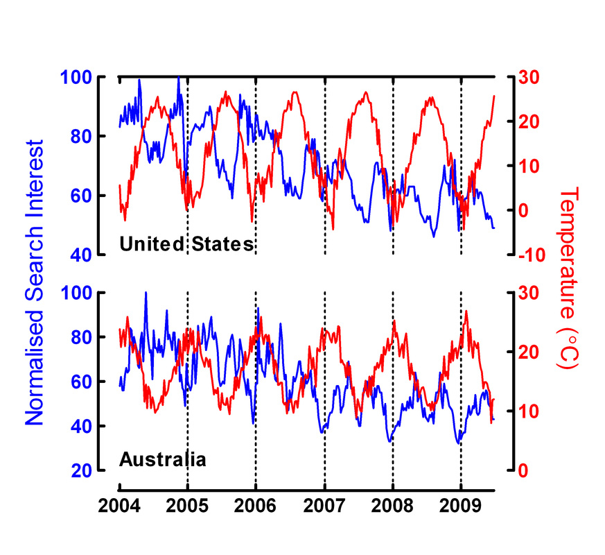
Using EMD method, we isolated seasonal IMF between search trend of health-related queries for depression (blue line) and temperature (red line) in the northern hemisphere (United States) and the southern hemisphere (Australia). The seasonal IMFs of search trends in both countries are negatively correlated with annual fluctuations in temperature (USA: r=-0.872, p<0.001; Australia: r=-0.656, p<0.001). Taken together, these findings suggest that the environmental factor was significantly associated with the fluctuation of health-related search queries for depression (see Figure below).

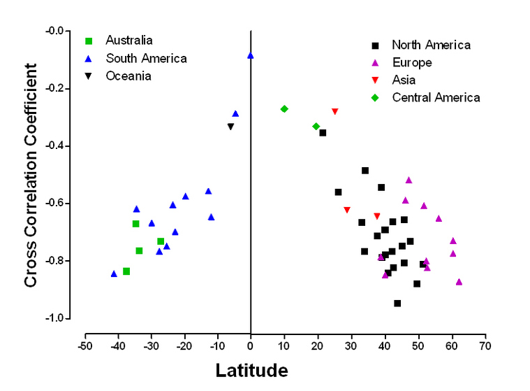
Next, we isolated seasonal IMFs of health-related search trends of depression in 54 geographic areas worldwide using EMD method. Based on cross correlation analysis between seasonal IMFs of search trends and temperature data, we found that the degree of correlation between searching for depression and temperature was latitude-dependent.
References
1. Yang AC*, Huang NE, Peng CK, Tsai SJ.* Do seasons have an influence on the incidence of depression? The use of an internet search engine query data as a proxy of human affect. PLoS ONE 5(10):e13728 (2010). [PDF]
2. Yang AC*, Tsai SJ, Huang NE. Decomposing the association of completed suicide with air pollution, weather, and unemployment data at different time scales. Journal of Affective Disorders 129:275-281 (2011).
Psychiatric News June 17, 2011 Volume 46 Number 12 Page 32: Breathing Polluted Air Linked to Suicide Risk
3. Yang AC, Fuh JL, Huang NE, Peng CK, Wang SJ.* Temporal associations between weather and headache: analysis by empirical mode decomposition. PLoS ONE 6(1):e14612 (2011). [PDF]
4. Yang AC*, Tsai SJ, Huang NE, Peng CK. Association of Internet search trends with suicide death in Taipei city, Taiwan, 2004-2009. Journal of Affective Disorders 132:179-184 (2011).
5. Yang AC, Fuh JL, Huang NE, Shia BC, Wang SJ*. Patients with migraine are right about their perception of temperature as a trigger - time series analysis of headache diary data. Journal of Headache & Pain. 16:533 (2015). [Full text]

|

|

|
Your comments and suggestions are welcome.
Please send your comments by email to Dr. Albert C. Yang (Laboratory of Precision Psychiatry).
Location: No. 155, Section 2, Linong Street, Beitou District, Taipei, Taiwan
Please send your comments by email to Dr. Albert C. Yang (Laboratory of Precision Psychiatry).
Location: No. 155, Section 2, Linong Street, Beitou District, Taipei, Taiwan